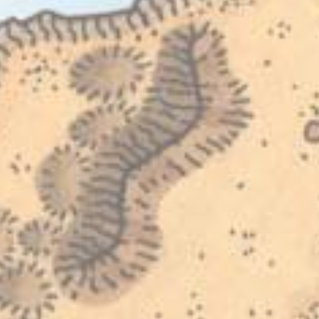
We are back in the mountain terrain. In the last post about it I was pretty confident with my approximation of its 3.5e visual style. However, “Theory and practice sometimes clash. And when that happens, theory loses. Every single time.” (L. Thorvalds, 2009). After trying out my design on more complex mountains, I found that tight turns of the flank geometry were rather common and caused notable fanning and self-intersections within the wide dotted flank lines. Even with significant manual optimization, the results were not really satisfactory. Drawing each flank line as an individual line object allows for more fine-grained control of the line placement at the cost of increasing the data size. Given that single mountains can contain hundreds of flank lines this increase might have some impact on the svg size, but at this point I do not see a way around it.

With that in mind, here are the new problems that need to be solved:

• Given an outline and a ridge, how can we place roughly evenly distributed lines between the two?
• How can we adjust these automatic lines to conform to the features on the drawn map?
• Come up with a way to annotate/generate the required data within an svg drawing software (i.e. Inkscape)

Connecting “Outer” and “Inner”

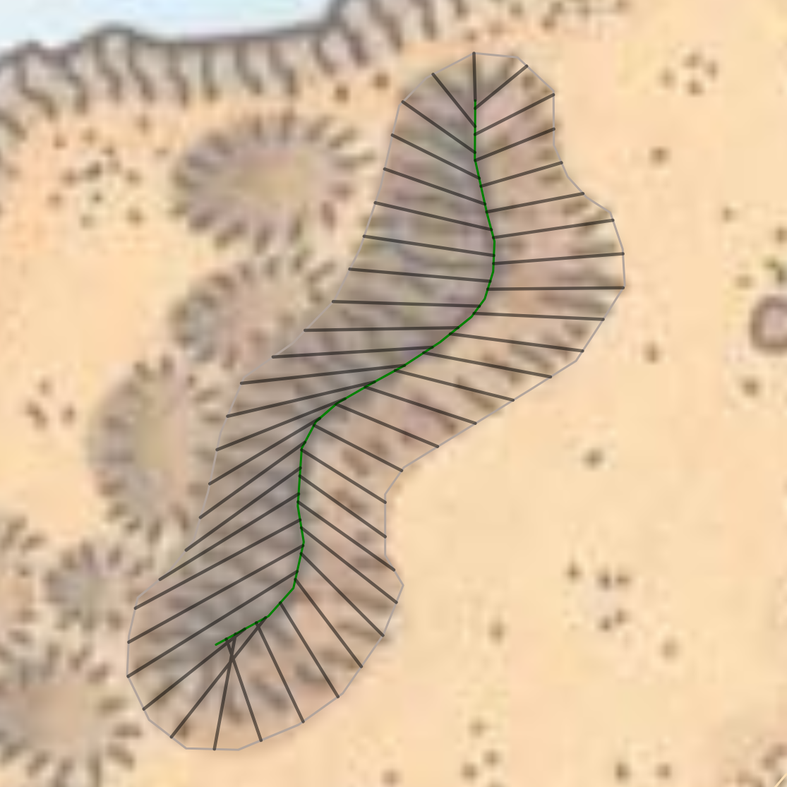
Going back to an uncomplicated example, a basic mountain is defined by an outline polygon and a polyline marking its ridge (We will ignore branching side ridges for now). Flank lines start at the outline, end at the ridge, and are placed roughly equidistant from each other while following the mountain’s shape. Notable exceptions are the ridge endpoints, where several flank lines join at (or at least very close to) the end of the polyline.

One way of simplifying this situation is to treat the ridge line as a polygon with no area. One side of this polygon follows the ridgeline from e.g. the upper endpoint to the lower one, and the other side follows the ridge in reverse, ending at the starting point. Now we have an outer and an inner polygon with the task to draw lines from one to the other. A naive approach would be to define a single flank line as starting point on the inner and outer polygons, then subdivide each polygon into the same number of pieces, and then draw the connections between these subdivisions.

It’s a decent start and, close to the starting flank, things seem to work. However, since the outer polygon does not perfectly follow the shape of the ridge, flank lines get out of sync the farther away they are from the defined starting point.

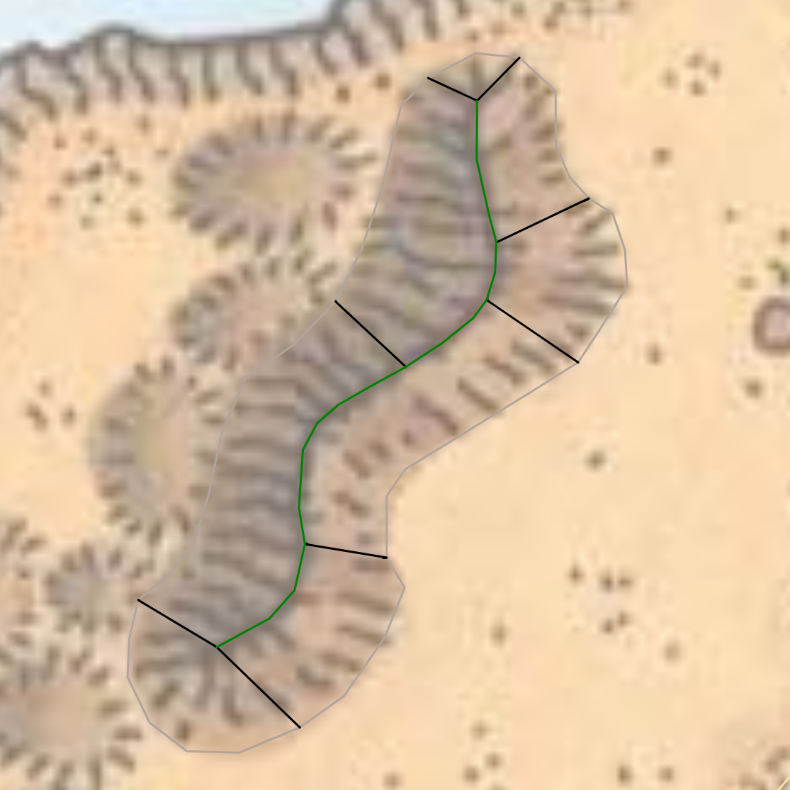
This is a problem in regions where the outline meanders a lot. At ridge endpoints, this naive approach does not allow multiple flank lines to end at a single point. We clearly need more control, so let’s add additional “guide” lines. This way we can split the inner and outer polygons into multiple sections. E.g., if the section on the ridge polygon is much shorter than on the outline, a fan-like flank line layout can be achieved.

Of course we now need to adjust the distance between flank lines based on the longer of inner and outer lines in each segment, to ensure a somewhat consistent placement. This makes the flank line spread more even, but the method isn’t failsafe.

In specific section geometries, adjacent lines might end up very close to each other and even line crossings can occur. This is particularly true once we need to handle branching ridgelines. Turf.js, the javascript library we are using for geospatial calculations, can help us to identify both of these situations with its built-in functions.

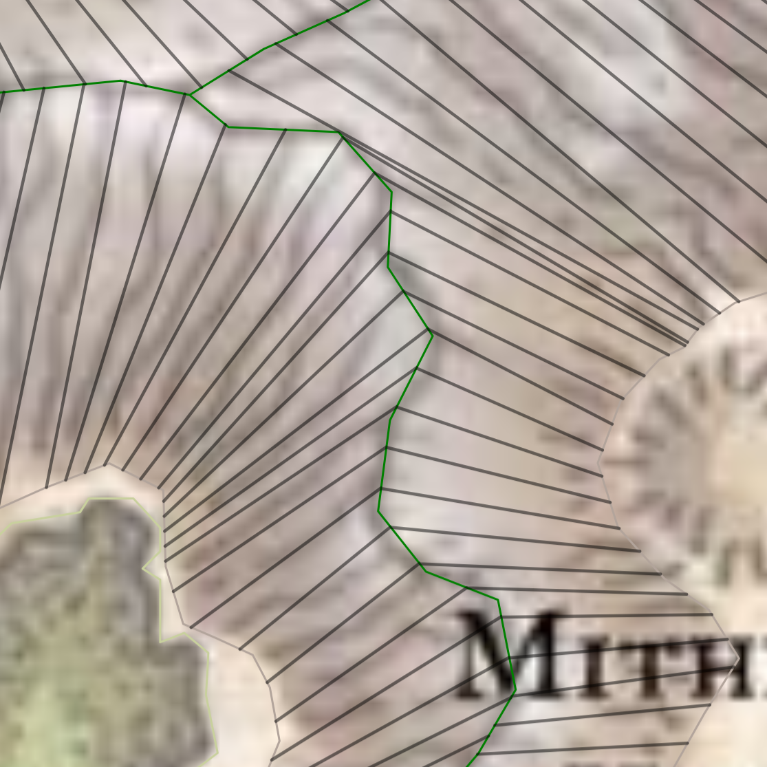
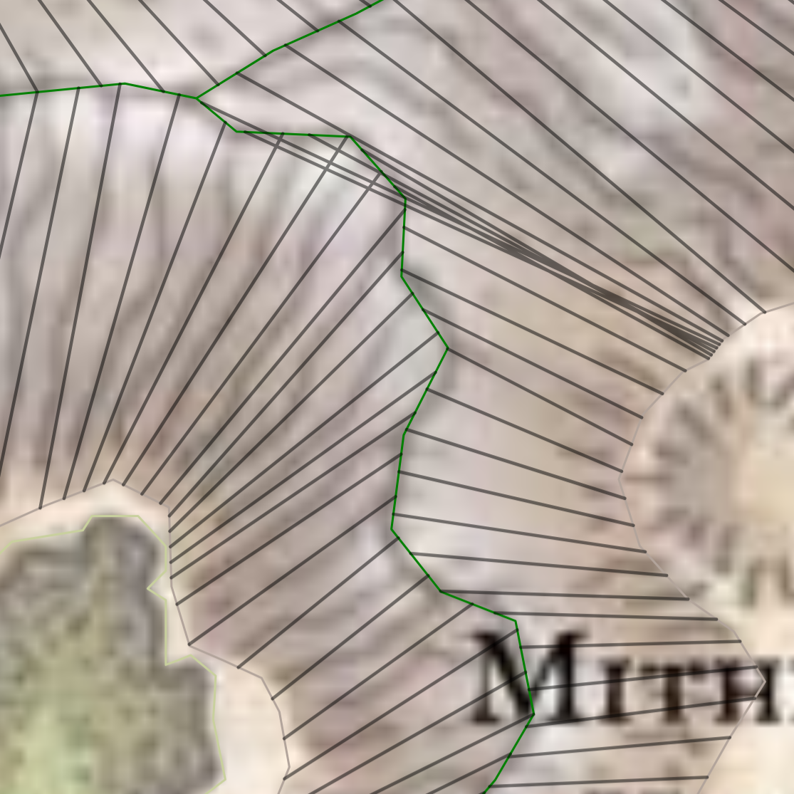
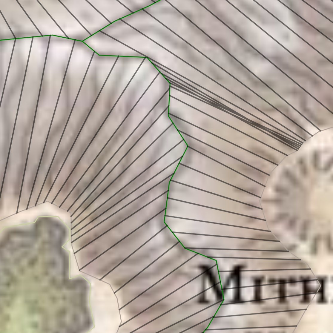
An initial adjustment is to trim flank lines that intersect with the ridge. This sometimes happens when the ridge has a very steep turnback, as in the example. To fix the situation we can trim the flank line back to the first intersection with the ridge. However, intersections with other flank lines need a different approach.

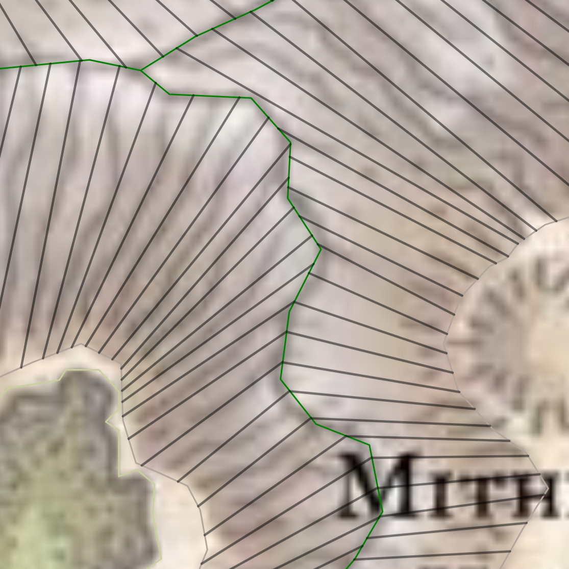
Before placing a new line, we compare it to the line preceding it. If an intersection is detected, we make a small adjustment step, i.e. 10% of the normal line offset, and try again. Eventually, we will find a line placement without crossing and continue as usual. This and various other situations may create flank lines that are nearly parallel and far closer than our target offset. As a final step, we also add adjustment steps at lines where both, the ridge AND the outline sides of the two lines are closer than 50% of the target offset. This still allows for fan shapes, since there only one side of the flank line pair is closer than 50%.

How to generate the data for this?

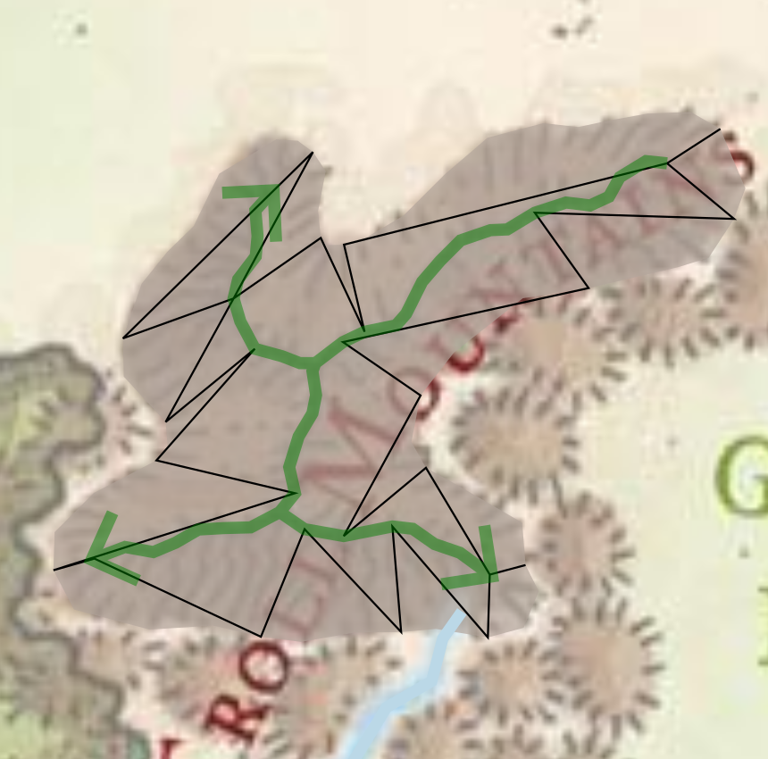
Since we don’t have a dedicated editor for all this map data (yet), we continue to use Inkscape to generate all data in svg format. We already have the mountain outlines and ridges, though for processing we add the convention that each mountain has a main ridge, and side ridges start from that main ridge and spread outwards. Instead of drawing flank guides as individual lines, we can simply connect all guides into a single linestring zig-zagging between outline and ridge. This way we can simplify creating multiple guides into one drawing operation.

What about shading?

Flank line positioning is only one part of the mountain style overall. We still have to take into account that flank lines are broken on the side of the mountain illuminated by the (virtual) sun. Since we are now dealing with individual lines, this is an easier task than before, but it will have to wait for the next post.